Building deep neural network - step by step

源链接:https://www.coursera.org/learn/neural-networks-deep-learning/ Week4 assignment(part 1 of 2)

  • 这周内容:实现所有建立深度神经网络需要的函数
  • 下周内容:构建用于图像分类的深度神经网络

本次作业的要求是

  • 用非线性单元(如:ReLU)来改进模型
  • 建立深度神经网络
  • 实现易于实用的神经网络

符号标记

  • 上标 $[l]$ 表示与第$l$层相关的量
    • 例:$a^{[L]}$是第$L$层激活层,$W^{[L]}$和$b^{[L]}$分别是第$L$层的参数。
  • 上标$(i)$表示与第$i$个样本相关的量
    • 例:$x^(i)$是第$i$个训练样本
  • 下标$i$表示某个向量的第$i$个量
    • 例:$a^{[l]}_i$表示第$l$个激活层的第$i$个元素

Packages

首先导入你需要用到的所有python库。

  • numpy
  • matplotlib
  • dnn_utils:提供了本文需要用到的一些必要的函数
  • testCases:提供了一些测试实例
  • np.random.seed(1)用来保证所有的随机函数都是一致的。
1
2
3
4
5
6
7
8
9
10
11
12
13
14
15
import numpy as np
import h5py
import matplotlib.pyplot as plt
from testCases import *
from dnn_utils import sigmoid, sigmoid_backward, relu, relu_backward
%matplotlib inline
plt.rcParams['figure.figsize'] = (5.0, 4.0) # set default size of plots
plt.rcParams['image.interpolation'] = 'nearest'
plt.rcParams['image.cmap'] = 'gray'
%load_ext autoreload
%autoreload 2
np.random.seed(1)

Outline of the Assignment

  • 初始化两层神经网络和$L$层神经网络的参数
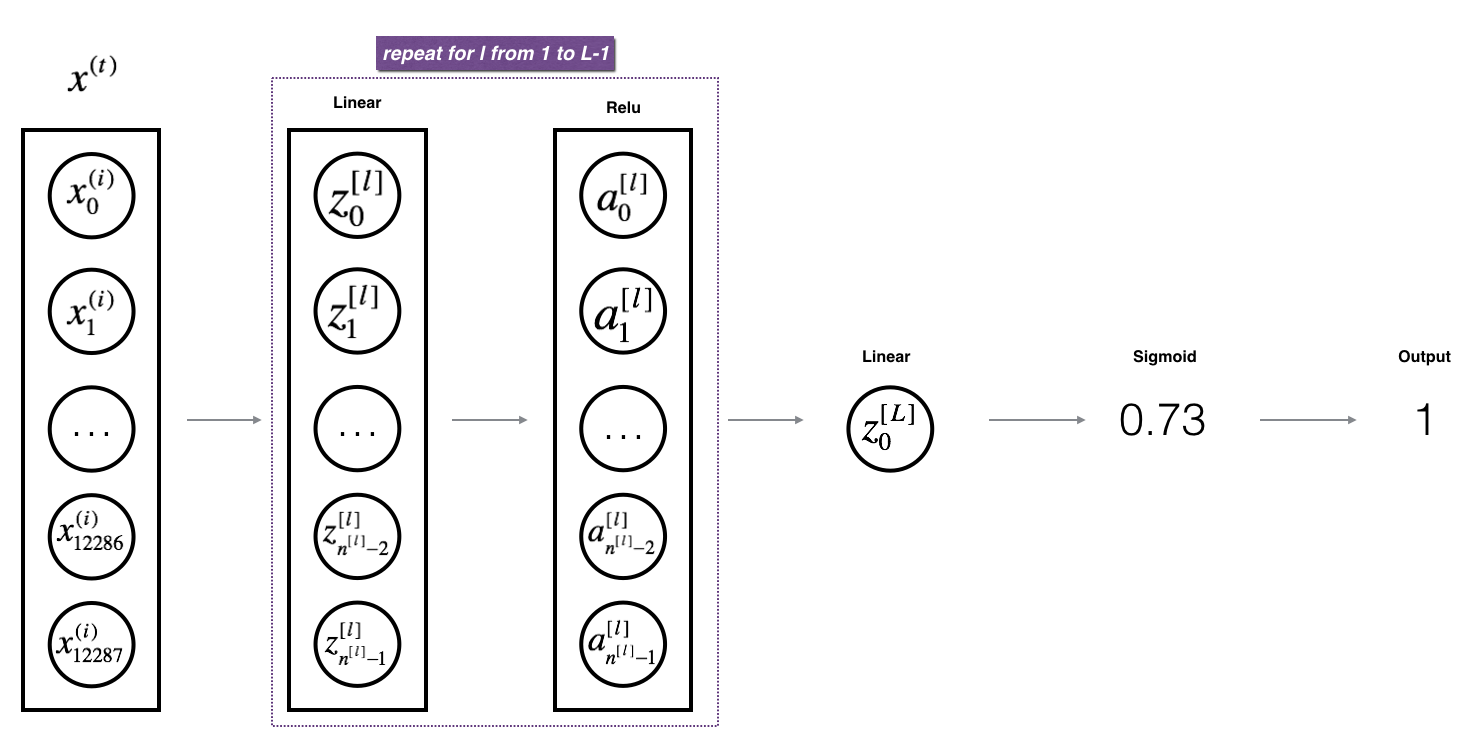
  • 实现前向传播模块(forward propagation module)
    • 实现某一层前向传播的线性部分(LINEAR)(结果为$Z^{[l]}$)
    • 给定激活函数ACTIVATION(relu/sigmoid)
    • 结合前两步实现新的[LINEAR->ACTIVATION]前向函数
    • 堆叠[LINEAR->ACTIVATION]前向函数$L-1$次(从第1层到第$L-1$层,在结尾加上[LINEAR->SIGMOID]作为最后第$L$层),则得到新的函数 L_model_forward。
  • 计算损失
  • 实现后向传播模块
    • 计算某一层后向传播的线性部分LINEAR。
    • 给定激活函数ACTIVATION的梯度(relu_backward/sigmoid_backward)。
    • 结合前面两步得到新的后向函数[LINEAR->ACTIVATION]。
    • 堆叠[LINEAR->ACTIVATION]后向函数$L-1$次,并加入[LINEAR->SIGMOID]后向函数,得到新的函数 L_model_backward。
  • 最后更新参数。

Initialization

下文实现了两个初始化的函数,第一个是用来初始化两层神经网络,第二个是$L$层神经网络。

2-lay Neural Network

Exercise: 创建并初始化二层神经网络

Instructions:

  • 模型结构是LINEAR->RELU->LINEAR->SIGMOID
  • 权重矩阵随机初始化,用:np.random.randn(shape)*0.01
  • 偏差初始化为0: mp.zeros(shape)
1
2
3
4
5
6
7
8
9
10
11
12
13
14
15
16
17
18
19
20
21
22
23
24
25
26
27
28
29
30
31
32
33
34
35
36
37
# GRADED FUNCTION: initialize_parameters
def initialize_parameters(n_x, n_h, n_y):
"""
Argument:
n_x -- size of the input layer
n_h -- size of the hidden layer
n_y -- size of the output layer
Returns:
parameters -- python dictionary containing your parameters:
W1 -- weight matrix of shape (n_h, n_x)
b1 -- bias vector of shape (n_h, 1)
W2 -- weight matrix of shape (n_y, n_h)
b2 -- bias vector of shape (n_y, 1)
"""
np.random.seed(1)
### START CODE HERE ### (≈ 4 lines of code)
W1 = np.random.randn(n_h, n_x) * 0.01
b1 = np.zeros(shape=(n_h, 1))
W2 = np.random.randn(n_y, n_h) * 0.01
b2 = np.zeros(shape=(n_y, 1))
### END CODE HERE ###
assert(W1.shape == (n_h, n_x))
assert(b1.shape == (n_h, 1))
assert(W2.shape == (n_y, n_h))
assert(b2.shape == (n_y, 1))
parameters = {"W1": W1,
"b1": b1,
"W2": W2,
"b2": b2}
return parameters
1
2
3
4
5
parameters = initialize_parameters(2,2,1)
print("W1 = " + str(parameters["W1"]))
print("b1 = " + str(parameters["b1"]))
print("W2 = " + str(parameters["W2"]))
print("b2 = " + str(parameters["b2"]))

Expected output:

name value
W1 [[ 0.01624345 -0.00611756] [-0.00528172 -0.01072969]]
W2 [[ 0.00865408 -0.02301539]]
b1 [[ 0.] [ 0.]]
b2 [[ 0.]]

L-layer Neural Network

L层神经网络的初始化要相对复杂一些。初始化的时候要注意匹配每一层的维度,$n^{[l]}$表示第$l$层的神经元数量,如果输入$X$是$(12288,209)$(有209个训练样本),则:

shape of W shape of b Activation Shape of Activation
Layer1 $(n^{[1]},12288)$ $(n^{[1]},1)$ $Z^{[1]}=W^{[1]}X+b^{[1]}$ $(n^{[1]},209)$
Layer2 $(n^{[2]},n^{[1]})$ $(n^{[2]},1)$ $Z^{[2]}=W^{[2]}A^{[1]}+b^{[2]}$ $(n^{[2]},209)$
Layer L-1 $(n^{[L-1]},n^{[L-2]})$ $(n^{[L-1]},1)$ $Z^{[L-1]}=W^{[L-1]}A^{[L-2]}+b^{[L-1]}$ $(n^{[L-1]},209)$
Layer L $(n^{[L]},n^{[L-1]})$ $(n^{[L]},1)$ $Z^{[L]}=W^{[L]}A^{[L-1]}+b^{[L]}$ $(n^{[L]},209)$

需要注意的是,由于python的broadcast特性,如果计算 WX+b,最后得到的结果是:
$$W = \begin{bmatrix} j & k & l \\ m & n & o \\ p & q & r \end{bmatrix},
X = \begin{bmatrix} a & b & c \\ d & e & f \\ g & h & i \end{bmatrix},
b = \begin{bmatrix} s \\ t \\ u \end{bmatrix}$$
$$WX+b = \begin{bmatrix} (ja+kd+lg)+s & (jb+ke+lh)+s & (jc+kf+li)+s \\
(ma+nd+og)+t & (mb+ne+oh)+t & (mc+nf+oi)+t \\
(pa+qd+rg)+u & (pb+qe+rh)+u & (pc+qf+ri)+u\end{bmatrix}$$

Excercise 实现L层神经网络的初始化

Instructions:

  • 模型结构是[LINEAR->RELU] × (L-1)->LINEAR->SIGMOID. 由L-1层RELU激活函数和带有sigmoid函数的输出层构成。
  • 权重矩阵随机初始化,采用np.random.rand(shape)*0.01
  • 偏差向量零初始化,采用np.zeros(shape)
  • 神经网络不同层的单元数储存在变量layer_dims中,例如,如果layer_dims的值为[2,4,1],则神经网络输入神经元有2个,隐层有4个神经元,输出层有1个神经元,也意味着W1的维度为(4,2),b1(4,1)W2(1,4),b2(1,1)
1
2
3
4
5
6
7
8
9
10
11
12
13
14
15
16
17
18
19
20
21
22
23
24
25
26
27
28
# GRADED FUNCTION: initialize_parameters_deep
def initialize_parameters_deep(layer_dims):
"""
Arguments:
layer_dims -- python array (list) containing the dimensions of each layer in our network
Returns:
parameters -- python dictionary containing your parameters "W1", "b1", ..., "WL", "bL":
Wl -- weight matrix of shape (layer_dims[l], layer_dims[l-1])
bl -- bias vector of shape (layer_dims[l], 1)
"""
np.random.seed(3)
parameters = {}
L = len(layer_dims) # number of layers in the network
for l in range(1, L):
### START CODE HERE ### (≈ 2 lines of code)
parameters['W' + str(l)] = np.random.randn(layer_dims[l], layer_dims[l - 1]) * 0.01
parameters['b' + str(l)] = np.zeros((layer_dims[l], 1))
### END CODE HERE ###
assert(parameters['W' + str(l)].shape == (layer_dims[l], layer_dims[l - 1]))
assert(parameters['b' + str(l)].shape == (layer_dims[l], 1))
return parameters
1
2
3
4
5
parameters = initialize_parameters_deep([5,4,3])
print("W1 = " + str(parameters["W1"]))
print("b1 = " + str(parameters["b1"]))
print("W2 = " + str(parameters["W2"]))
print("b2 = " + str(parameters["b2"]))

Expected output:

name value
W1 [[ 0.01788628 0.0043651 0.00096497 -0.01863493 -0.00277388] [-0.00354759 -0.00082741 -0.00627001 -0.00043818 -0.00477218] [-0.01313865 0.00884622 0.00881318 0.01709573 0.00050034] [-0.00404677 -0.0054536 -0.01546477 0.00982367 -0.01101068]]
b1 [[ 0.] [ 0.] [ 0.] [ 0.]]
W2 [[-0.01185047 -0.0020565 0.01486148 0.00236716] [-0.01023785 -0.00712993 0.00625245 -0.00160513] [-0.00768836 -0.00230031 0.00745056 0.01976111]]
b2 [[ 0.] [ 0.] [ 0.]]

Forward propagation module

Linear Forward

本模块按顺序实现了一下函数:

  • LINEAR
  • LINEAR->ACTIVATION,其中激活函数是ReLU或者Sigmoid
  • [LINEAR->RELU] × (L-1) -> LINEAR -> SIGMOID

线性前向模块主要实现如下公式:
$$Z^{[l]} = W^{[l]}A^{[l-1]}+b^{[l]}$$
其中$A^{[0]}=X$

Excersice: 实现前向传播的线性部分

1
2
3
4
5
6
7
8
9
10
11
12
13
14
15
16
17
18
19
20
21
22
def linear_forward(A, W, b):
"""
Implement the linear part of a layer's forward propagation.
Arguments:
A -- activations from previous layer (or input data): (size of previous layer, number of examples)
W -- weights matrix: numpy array of shape (size of current layer, size of previous layer)
b -- bias vector, numpy array of shape (size of the current layer, 1)
Returns:
Z -- the input of the activation function, also called pre-activation parameter
cache -- a python dictionary containing "A", "W" and "b" ; stored for computing the backward pass efficiently
"""
### START CODE HERE ### (≈ 1 line of code)
Z = np.dot(W, A) + b
### END CODE HERE ###
assert(Z.shape == (W.shape[0], A.shape[1]))
cache = (A, W, b)
return Z, cache
1
2
3
4
A, W, b = linear_forward_test_case()
Z, linear_cache = linear_forward(A, W, b)
print("Z = " + str(Z))

Linear-Activation Forward

本文将会用到两种激活函数:

  • Sigmoid: $\sigma(Z)=\sigma(WA+b)=\frac{1}{1+e^{-(WA+b)}}$,这个函数返回两项值:激活后的值’a’和包含’Z’的’cache’。调用方法为:
    A, activation_cache = sigmoid(Z)
  • ReLU:ReLU函数的数学形式是 $A=RELU(Z)=\max(0,Z)$,这个函数返回两项值:激活后的值’a’和包含’Z’的’cache’。调用方法为:
    A, activation_cache = relu(Z)

Excersice: 实现前向传播中的LINEAR->ACTIVATION层,即$A^{[l]}=g(Z^{[l]})=g(W^{[l]}A^{[l-1]}+b^{[l]})$,其中’g’可以是sigmoid()或者relu()。用linear_forward()和对应的激活函数。

1
2
3
4
5
6
7
8
9
10
11
12
13
14
15
16
17
18
19
20
21
22
23
24
25
26
27
28
29
30
31
32
33
34
35
36
# GRADED FUNCTION: linear_activation_forward
def linear_activation_forward(A_prev, W, b, activation):
"""
Implement the forward propagation for the LINEAR->ACTIVATION layer
Arguments:
A_prev -- activations from previous layer (or input data): (size of previous layer, number of examples)
W -- weights matrix: numpy array of shape (size of current layer, size of previous layer)
b -- bias vector, numpy array of shape (size of the current layer, 1)
activation -- the activation to be used in this layer, stored as a text string: "sigmoid" or "relu"
Returns:
A -- the output of the activation function, also called the post-activation value
cache -- a python dictionary containing "linear_cache" and "activation_cache";
stored for computing the backward pass efficiently
"""
if activation == "sigmoid":
# Inputs: "A_prev, W, b". Outputs: "A, activation_cache".
### START CODE HERE ### (≈ 2 lines of code)
Z, linear_cache = linear_forward(A_prev, W, b)
A, activation_cache = sigmoid(Z)
### END CODE HERE ###
elif activation == "relu":
# Inputs: "A_prev, W, b". Outputs: "A, activation_cache".
### START CODE HERE ### (≈ 2 lines of code)
Z, linear_cache = linear_forward(A_prev, W, b)
A, activation_cache = relu(Z)
### END CODE HERE ###
assert (A.shape == (W.shape[0], A_prev.shape[1]))
cache = (linear_cache, activation_cache)
return A, cache
1
2
3
4
5
6
7
A_prev, W, b = linear_activation_forward_test_case()
A, linear_activation_cache = linear_activation_forward(A_prev, W, b, activation = "sigmoid")
print("With sigmoid: A = " + str(A))
A, linear_activation_cache = linear_activation_forward(A_prev, W, b, activation = "relu")
print("With ReLU: A = " + str(A))

L-layer model

对于有L层的神经网络来说,前向传播由L-1个linear_activation_forwardwith RELU和一个linear_activation_forwardwith SIGMOID构成。

Excersice:实现上述模型的前向传播

1
2
3
4
5
6
7
8
9
10
11
12
13
14
15
16
17
18
19
20
21
22
23
24
25
26
27
28
29
30
31
32
33
34
35
36
37
38
39
40
41
42
43
44
45
46
47
# GRADED FUNCTION: L_model_forward
def L_model_forward(X, parameters):
"""
Implement forward propagation for the [LINEAR->RELU]*(L-1)->LINEAR->SIGMOID computation
Arguments:
X -- data, numpy array of shape (input size, number of examples)
parameters -- output of initialize_parameters_deep()
Returns:
AL -- last post-activation value
caches -- list of caches containing:
every cache of linear_relu_forward() (there are L-1 of them, indexed from 0 to L-2)
the cache of linear_sigmoid_forward() (there is one, indexed L-1)
"""
caches = []
A = X
L = len(parameters) // 2 # number of layers in the neural network
# Implement [LINEAR -> RELU]*(L-1). Add "cache" to the "caches" list.
for l in range(1, L):
A_prev = A
### START CODE HERE ### (≈ 2 lines of code)
A, cache = linear_activation_forward(A_prev,
parameters['W' + str(l)],
parameters['b' + str(l)],
activation='relu')
caches.append(cache)
### END CODE HERE ###
# Implement LINEAR -> SIGMOID. Add "cache" to the "caches" list.
### START CODE HERE ### (≈ 2 lines of code)
AL, cache = linear_activation_forward(A,
parameters['W' + str(L)],
parameters['b' + str(L)],
activation='sigmoid')
caches.append(cache)
### END CODE HERE ###
assert(AL.shape == (1, X.shape[1]))
return AL, caches
`
1
2
3
4
X, parameters = L_model_forward_test_case()
AL, caches = L_model_forward(X, parameters)
print("AL = " + str(AL))
print("Length of caches list = " + str(len(caches)))

Cost function

Excersice:计算交叉熵损失(cross-entropy cost)$J$,公式如下:
$$-\frac{1}{m} \sum\limits_{i = 1}^{m} (y^{(i)}\log\left(a^{[L] (i)}\right) + (1-y^{(i)})\log\left(1- a^{[L] (i)}\right))$$

1
2
3
4
5
6
7
8
9
10
11
12
13
14
15
16
17
18
19
20
21
22
23
24
25
# GRADED FUNCTION: compute_cost
def compute_cost(AL, Y):
"""
Implement the cost function defined by equation (7).
Arguments:
AL -- probability vector corresponding to your label predictions, shape (1, number of examples)
Y -- true "label" vector (for example: containing 0 if non-cat, 1 if cat), shape (1, number of examples)
Returns:
cost -- cross-entropy cost
"""
m = Y.shape[1]
# Compute loss from aL and y.
### START CODE HERE ### (≈ 1 lines of code)
cost = (-1 / m) * np.sum(np.multiply(Y, np.log(AL)) + np.multiply(1 - Y, np.log(1 - AL)))
### END CODE HERE ###
cost = np.squeeze(cost) # To make sure your cost's shape is what we expect (e.g. this turns [[17]] into 17).
assert(cost.shape == ())
return cost
1
2
3
Y, AL = compute_cost_test_case()
print("cost = " + str(compute_cost(AL, Y)))

Backward propagation module

Reminder:

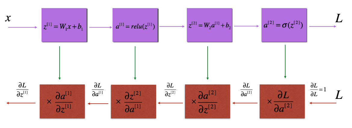
与前向传播类似,后向传播的实现也分成三个步骤:

  • LINEAR backward
  • LINEAR->ACTIVATION backward,其中ACTIVATION是ReLU或者sigmoid函数
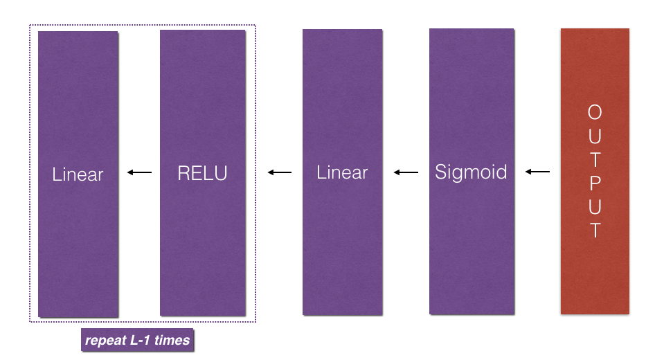
  • [LINEAR->RELU]× (L-1)->LINEAR->SIGMOID backward

Linear backward

对于第l层神经网络,线性部分是:$Z^{[l]} = W^{[l]}A^{[l-1]}+b^{[l]}$。假设已知$d Z^{[l]} = \frac{\partial L}{\partial Z^{[l]}}$,需要求的是 $dW^{[l]}$, $db^{[l]}$以及$dA^{[l-1]}$。

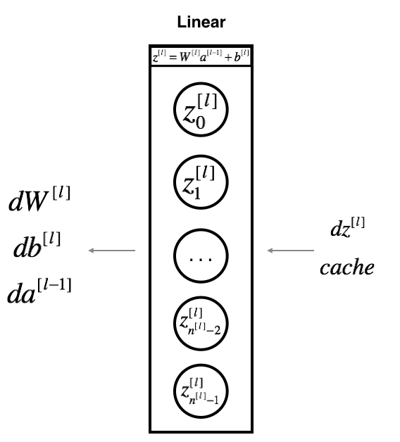
三个输出$dW^{[l]}$, $db^{[l]}$以及$dA^{[l-1]}$可以用输入$d Z^{[l]}$ 来计算:

$$dW^{[l]}=\frac{\partial L}{\partial W^{[l]}} = \frac{1}{m}d Z^{[l]}A^{[l-1]T}$$

$$ db^{[l]}=\frac{\partial L}{\partial b^{[l]}} = \frac{1}{m} \sum^m_{i=1}dZ^{[l] (i)} $$

$$dA^{[l-1]} = \frac{\partial L}{\partial A^{[l-1]}} = W^{[l]T}dZ^{[l]}$$

1
2
3
4
5
6
7
8
9
10
11
12
13
14
15
16
17
18
19
20
21
22
23
24
25
26
27
28
def linear_backward(dZ, cache):
"""
Implement the linear portion of backward propagation for a single layer (layer l)
Arguments:
dZ -- Gradient of the cost with respect to the linear output (of current layer l)
cache -- tuple of values (A_prev, W, b) coming from the forward propagation in the current layer
Returns:
dA_prev -- Gradient of the cost with respect to the activation (of the previous layer l-1), same shape as A_prev
dW -- Gradient of the cost with respect to W (current layer l), same shape as W
db -- Gradient of the cost with respect to b (current layer l), same shape as b
"""
A_prev, W, b = cache
m = A_prev.shape[1]
### START CODE HERE ### (≈ 3 lines of code)
dW = np.dot(dZ, cache[0].T) / m
db = np.squeeze(np.sum(dZ, axis=1, keepdims=True)) / m
dA_prev = np.dot(cache[1].T, dZ)
### END CODE HERE ###
assert (dA_prev.shape == A_prev.shape)
assert (dW.shape == W.shape)
assert (isinstance(db, float))
return dA_prev, dW, db
1
2
3
4
5
6
7
# Set up some test inputs
dZ, linear_cache = linear_backward_test_case()
dA_prev, dW, db = linear_backward(dZ, linear_cache)
print ("dA_prev = "+ str(dA_prev))
print ("dW = " + str(dW))
print ("db = " + str(db))

Linear-Activation backward

  • sigmoid_backward 实现了SIGMOID函数的后向传播,调用方法:
    dZ = sigmoid_backward(dA, activation_cache)

  • relu_backward 实现了relu函数的后向传播,调用方法:
    dZ = relu_backward(dA, activation_cache)

如果$g(.)$是激活函数,sigmoid_backward和relu_backward的计算是:
$$dZ^{[l]} = dA^{[l]}*g’(Z^{[l]})$$

Excersice:实现LINEAR->ACTIVATION层的后向传播:

1
2
3
4
5
6
7
8
9
10
11
12
13
14
15
16
17
18
19
20
21
22
23
24
25
26
27
28
29
30
def linear_activation_backward(dA, cache, activation):
"""
Implement the backward propagation for the LINEAR->ACTIVATION layer.
Arguments:
dA -- post-activation gradient for current layer l
cache -- tuple of values (linear_cache, activation_cache) we store for computing backward propagation efficiently
activation -- the activation to be used in this layer, stored as a text string: "sigmoid" or "relu"
Returns:
dA_prev -- Gradient of the cost with respect to the activation (of the previous layer l-1), same shape as A_prev
dW -- Gradient of the cost with respect to W (current layer l), same shape as W
db -- Gradient of the cost with respect to b (current layer l), same shape as b
"""
linear_cache, activation_cache = cache
if activation == "relu":
### START CODE HERE ### (≈ 2 lines of code)
dZ = relu_backward(dA, activation_cache)
### END CODE HERE ###
elif activation == "sigmoid":
### START CODE HERE ### (≈ 2 lines of code)
dZ = sigmoid_backward(dA, activation_cache)
### END CODE HERE ###
# Shorten the code
dA_prev, dW, db = linear_backward(dZ, linear_cache)
return dA_prev, dW, db
1
2
3
4
5
6
7
8
9
10
11
12
13
AL, linear_activation_cache = linear_activation_backward_test_case()
dA_prev, dW, db = linear_activation_backward(AL, linear_activation_cache, activation = "sigmoid")
print ("sigmoid:")
print ("dA_prev = "+ str(dA_prev))
print ("dW = " + str(dW))
print ("db = " + str(db) + "\n")
dA_prev, dW, db = linear_activation_backward(AL, linear_activation_cache, activation = "relu")
print ("relu:")
print ("dA_prev = "+ str(dA_prev))
print ("dW = " + str(dW))
print ("db = " + str(db))

L-Model backward

当实现L_model_forward函数时,在每次迭代中都保存了(X,W,b,Z)的值,在后向传播模块中,你将用到这些值来计算梯度。

Initializing backpropagation: 上述网络的输出是:$A^{[L]} = \sigma(Z^{[L]})$。因此需要计算$dAL = \frac{\partial L}{\partial A^{[L]}}$.

dAL = - (np.divide(Y, AL) - np.divide(1 - Y, 1 - AL))

Excercise:实现后向传播:[LINEAR->RELU] × (l-1) -> LINEAR -> SIGMOID 模型。

1
2
3
4
5
6
7
8
9
10
11
12
13
14
15
16
17
18
19
20
21
22
23
24
25
26
27
28
29
30
31
32
33
34
35
36
37
38
39
40
41
42
43
44
45
46
47
def L_model_backward(AL, Y, caches):
"""
Implement the backward propagation for the [LINEAR->RELU] * (L-1) -> LINEAR -> SIGMOID group
Arguments:
AL -- probability vector, output of the forward propagation (L_model_forward())
Y -- true "label" vector (containing 0 if non-cat, 1 if cat)
caches -- list of caches containing:
every cache of linear_activation_forward() with "relu" (it's caches[l], for l in range(L-1) i.e l = 0...L-2)
the cache of linear_activation_forward() with "sigmoid" (it's caches[L-1])
Returns:
grads -- A dictionary with the gradients
grads["dA" + str(l)] = ...
grads["dW" + str(l)] = ...
grads["db" + str(l)] = ...
"""
grads = {}
L = len(caches) # the number of layers
m = AL.shape[1]
Y = Y.reshape(AL.shape) # after this line, Y is the same shape as AL
# Initializing the backpropagation
### START CODE HERE ### (1 line of code)
dAL = dAL = - (np.divide(Y, AL) - np.divide(1 - Y, 1 - AL))
### END CODE HERE ###
# Lth layer (SIGMOID -> LINEAR) gradients. Inputs: "AL, Y, caches". Outputs: "grads["dAL"], grads["dWL"], grads["dbL"]
### START CODE HERE ### (approx. 2 lines)
current_cache = caches[-1]
grads["dA" + str(L)], grads["dW" + str(L)], grads["db" + str(L)] = linear_backward(sigmoid_backward(dAL,
current_cache[1]),
current_cache[0])
### END CODE HERE ###
for l in reversed(range(L-1)):
# lth layer: (RELU -> LINEAR) gradients.
# Inputs: "grads["dA" + str(l + 2)], caches". Outputs: "grads["dA" + str(l + 1)] , grads["dW" + str(l + 1)] , grads["db" + str(l + 1)]
### START CODE HERE ### (approx. 5 lines)
current_cache = caches[l]
dA_prev_temp, dW_temp, db_temp = linear_backward(sigmoid_backward(dAL, caches[1]), caches[0])
grads["dA" + str(l + 1)] = dA_prev_temp
grads["dW" + str(l + 1)] = dW_temp
grads["db" + str(l + 1)] = db_temp
### END CODE HERE ###
return grads
1
2
3
4
5
X_assess, Y_assess, AL, caches = L_model_backward_test_case()
grads = L_model_backward(AL, Y_assess, caches)
print ("dW1 = "+ str(grads["dW1"]))
print ("db1 = "+ str(grads["db1"]))
print ("dA1 = "+ str(grads["dA1"]))

Update parameters

在这一节,你将用梯度下降法更新模型参数:
$$b^{[l]} = b^{[l]} - \alpha db^{[l]}$$
其中$\alpha$是学习率。

Excercise:实现update_parameters()函数

1
2
3
4
5
6
7
8
9
10
11
12
13
14
15
16
17
18
19
20
21
22
23
24
def update_parameters(parameters, grads, learning_rate):
"""
Update parameters using gradient descent
Arguments:
parameters -- python dictionary containing your parameters
grads -- python dictionary containing your gradients, output of L_model_backward
Returns:
parameters -- python dictionary containing your updated parameters
parameters["W" + str(l)] = ...
parameters["b" + str(l)] = ...
"""
L = len(parameters) // 2 # number of layers in the neural network
# Update rule for each parameter. Use a for loop.
### START CODE HERE ### (≈ 3 lines of code)
for l in range(L):
parameters["W" + str(l + 1)] = parameters["W" + str(l + 1)] - learning_rate * grads["dW" + str(l + 1)]
parameters["b" + str(l + 1)] = parameters["b" + str(l + 1)] - learning_rate * grads["db" + str(l + 1)]
### END CODE HERE ###
return parameters
1
2
3
4
5
6
7
8
9
parameters, grads = update_parameters_test_case()
parameters = update_parameters(parameters, grads, 0.1)
print ("W1 = " + str(parameters["W1"]))
print ("b1 = " + str(parameters["b1"]))
print ("W2 = " + str(parameters["W2"]))
print ("b2 = " + str(parameters["b2"]))
print ("W3 = " + str(parameters["W3"]))
print ("b3 = " + str(parameters["b3"]))